
Access the full suite of ESA Climate Change Initiative data products via our dedicate Open Data Portal, including those generated by the CCI Glaciers project.
The main products are glacier outlines and inventories, elevation and mass changes, and maps of flow velocities. They can be downloaded from a dedicated website hosted by ENVEO. Apart from creating datasets, a major effort has been and is spent on publications that are providing in-depth information about several of the produced datasets, the algorithms applied and the lessons learned. The studies range from change assessment over large regions to detailed investigations of individual glaciers. Below we shortly describe the methods used to generate the datasets. Further details can be found in the ATBD.
1. Glacier Outlines and Inventories
We are using multispectral optical satellite data (mostly Landsat and Sentinel-2) and a simple band ratio with a threshold to create binary maps of clean ice. This method works very well as glacier ice and snow have large differences in spectral reflectance in the visible and near infrared (VNIR) compared to the shortwave infrared (SWIR). The binary maps are converted from raster to vector format and are edited manually by visual inspection using a range of colour composites of the same image in the background. The main issues are that debris-covered ice is not mapped but should be included (omission errors) whereas ice bergs, sea ice or turbid water is included but should not (commission errors). For a better identification of debris-covered glaciers, we also consider coherence images from SAR sensors (ALOS PALSAR, Sentinel-1) that often reveal the moving parts of a glacier with extraordinary clarity.
Once outlines are corrected, they are digitally intersected with drainage divides derived by watershed modelling from a digital elevation model (DEM). The same DEM is finally used to determine for each glacier polygon a series of topographic parameters (e.g. minimum, maximum and median elevation, mean slope and aspect) as required for a glacier inventory. The finalized dataset is then submitted to the GLIMS glacier database. Current research has a focus on a more automated mapping of debris-covered glaciers and cloud-based processing of image stacks to avoid scene-by-scene processing and laborious mosaicking of results (e.g. in regions that are often cloud-covered).
Randolph Glacier Inventory version 5.0 - interactive globe
2. Elevation Changes
We utilize several methods to determine elevation changes of the glacier surface. These include repeat altimetry from optical (e.g. ICESat) and radar (e.g. Cryosat-2) sensors, comparison of altimetry data to a DEM (e.g. SRTM) or differencing of DEMs from two points in time (e.g. TanDEM-X – SRTM). Current techniques (=> link ) use stacks of multiple DEMs generated automatically from stereo sensors to derive more robust trends in elevation change for each DEM cell. Three critical points to consider before volume changes of entire glaciers can be derived from the datasets are (1) proper co-registration (a pre-processing step), (2) handling of artefacts and outliers and (3) spatial interpolation of data voids and uncovered regions (both post-processing steps). Whereas for issue (1) automated methods are in place (=> link ), issues (2) and (3) have to be solved individually by considering the highly variable nature of these issues. Many studies use filters (an elevation change threshold) to remove outliers and mean values of elevation changes as derived for specific elevation bands to extrapolate data voids (=> link).
However, these methods are not standardized so that different authors would obtain slightly different results for the same dataset. Another issue requiring attention is radar penetration when using DEMs obtained from InSAR (e.g. SRTM or TanDEM-X). Penetration into dry snow and firn varies with the band (e.g. is stronger for C than for X band) and the specific dielectric properties of the surface (e.g. moisture content). As the latter are generally unknown and can be locally highly variable, a standard correction might not provide the best results. Current research aims at a better determination of radar penetration, improved artefact handling and data void interpolation as well as completing global coverage.
3. Flow velocities
Glacier flow velocities can be derived automatically from repeat satellite imagery using offset tracking (optical & SAR) and interferometric techniques (SAR only). Synthetic Aperture Radar (SAR) data, over optical, has the advantage of being applicable all-year and in all-weather conditions. The InSAR technique has the highest accuracy, but requires satellite data from crossing orbits (e.g. ascending and descending) and usually works best only in comparably slow moving and flat terrain. The use of optical imagery requires visible surface features that can be tracked, so good contrast and limited self-similarity is essential. It is thus working better for ablation regions of glaciers than for snow-covered areas with little contrast. Unreliable data are filtered, causing data voids in the flow field that can partly be filled by processing several scene pairs and stacking them. Dynamically instable, small, fast flowing or surging glaciers are challenging for all techniques but are a key focus in this project.
Recent methodological advances and increased satellite coverage now allow for continuous retrieval of ice velocities over short periods (down to 6-12 days with Sentinel-1). This enables the monitoring of ice flow even on fast-flowing and surging glaciers, revealing precious insights into flow governing processes. Several studies by Glaciers CCI team members have investigated the related methods (=> link) and applied them to surging glaciers in HMA (=> link) or the Arctic (=> link). For the latter region SAR data are of particular importance as polar night and frequent cloud cover prevents continuous observations with optical sensors. The 6-day repeat period of Sentinel-1 is of special advantage as the short interval reduces decorrelation and provides more complete flow fields. Current methodological research has a focus on the combination of multiple sensors and a better consideration of smaller glaciers.
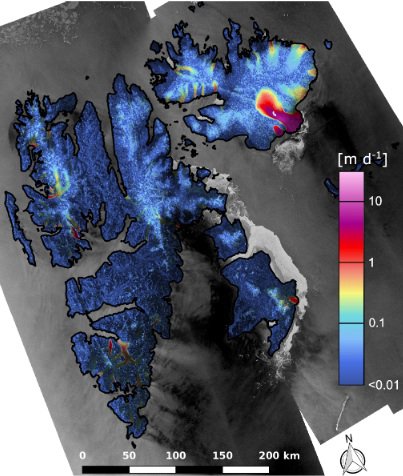
Figure 1: Glacier velocity in Svalbard derived from Sentinel-1 data. Image credit: contains modified Copernicus Sentinel-1 data (2016), processed by ENVEO.